
This course introduces the basic concepts and methods of geostatistics for understanding and analyzing spatial variability in geological data. Students will learn about regionalized variables, variogram analysis, and kriging for mapping geological properties. Practical exercises focus on variogram computation and spatial interpolation to support fundamental geological studies.
- Enseignant: Rabah KECHICHED
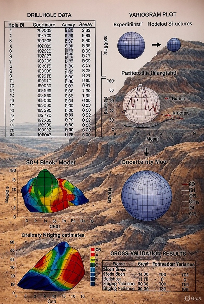
Geostatistics focuses on analyzing, modeling, and predicting phenomena that vary across space or time. Developed initially in the mining and petroleum industries, it provides powerful tools for understanding the spatial continuity of geological variables such as grade, porosity, permeability, and facies distribution. By combining probability theory with spatial data analysis, geostatistics helps quantify uncertainty and produce more accurate maps and models of the subsurface.
- Enseignant: Rabah KECHICHED
Statement
Using the geochemical dataset provided below, you are required to perform the following statistical analyses:
Univariate Statistics (to be completed before 23/10/2025)
1. Prepare a statistical summary table for two selected elements.
2. Compute the statistical parameters of central tendency and dispersion, and provide a brief interpretation.
3. Construct the relative and cumulative frequency histograms for the two selected variables.
4. Plot the probability graph (Henry line), identify potential sub-populations, and provide comments.
Bivariate Statistics (to be completed before 30/10/2025)
1. Plot the scatter diagram (x, y) on graph paper and interpret the distribution pattern of the data points.
2. Calculate the correlation coefficient (r).
3. Test its statistical significance using the formula R = 2/√(n-1).
4. Establish the simple linear regression equation Y = aX + B and draw the corresponding regression line.
Table – Geochemical Data (unit %)
|
N |
P2O5 |
CO2 |
MgO |
CaO |
SiO2 |
|
1 |
4 |
37 |
17 |
35 |
1 |
|
2 |
12 |
23 |
9 |
37 |
5 |
|
3 |
15 |
20 |
7 |
38 |
4 |
|
4 |
15 |
22 |
9 |
41 |
|
|
5 |
16 |
18 |
8 |
42 |
1 |
|
6 |
16 |
25 |
10 |
41 |
0 |
|
7 |
17 |
20 |
9 |
41 |
0 |
|
8 |
17 |
21 |
8 |
41 |
2 |
|
9 |
18 |
21 |
9 |
40 |
0 |
|
10 |
18 |
21 |
8 |
41 |
2 |
|
11 |
18 |
21 |
9 |
41 |
0 |
|
12 |
19 |
17 |
6 |
42 |
2 |
|
13 |
20 |
19 |
7 |
42 |
|
|
14 |
20 |
18 |
6 |
44 |
0 |
|
15 |
21 |
19 |
7 |
43 |
1 |
|
16 |
22 |
15 |
5 |
44 |
0 |
|
17 |
22 |
13 |
4 |
46 |
0 |
|
18 |
22 |
25 |
9 |
40 |
1 |
|
19 |
22 |
12 |
4 |
44 |
1 |
|
20 |
22 |
13 |
4 |
45 |
1 |
|
21 |
23 |
8 |
1 |
49 |
0 |
|
22 |
23 |
13 |
4 |
44 |
2 |
|
23 |
24 |
17 |
5 |
44 |
0 |
|
24 |
24 |
11 |
3 |
45 |
1 |
|
25 |
25 |
14 |
5 |
44 |
0 |
|
26 |
25 |
13 |
4 |
46 |
0 |
|
27 |
25 |
8 |
1 |
48 |
0 |
|
28 |
26 |
11 |
4 |
46 |
1 |
|
29 |
27 |
5 |
1 |
45 |
|
|
30 |
27 |
10 |
2 |
47 |
0 |
|
31 |
27 |
8 |
2 |
48 |
1 |
|
32 |
28 |
8 |
1 |
50 |
0 |
|
33 |
29 |
8 |
1 |
49 |
0 |
|
34 |
29 |
7 |
1 |
50 |
0 |
|
35 |
29 |
8 |
1 |
49 |
0 |
|
36 |
29 |
7 |
1 |
50 |
0 |
|
37 |
30 |
7 |
1 |
50 |
0 |
|
38 |
30 |
7 |
1 |
50 |
0 |
|
39 |
30 |
7 |
1 |
50 |
0 |
|
40 |
12 |
23 |
9 |
41 |
3 |

CHAPTER 1. REVIEW OF DATA ANALYSIS
1. Univariate Statistics
This analysis makes it possible to determine the statistical parameters describing the distribution of the studied variables (measures of central tendency and dispersion).
a) Measures of Central Tendency
These parameters quantify the central tendency of the values within a statistical series. The main measures of central tendency are the mode, the median, and the arithmetic mean.
• Mode (Mo): The mode is defined as the value of the random variable that has the highest frequency. A statistical series may be unimodal or multimodal. The number of modes in a statistical series provides information about the homogeneity or heterogeneity of the sample or population. However, in the case of grouped data, the number of modes may depend on the number of classes and the class interval.
• Median: The median is the value of the variable corresponding to a cumulative frequency of 50%.
• Arithmetic Mean (M or X̄): The arithmetic mean is equal to the sum of all values in the series divided by the total number of observations (N).
b) Measures of Dispersion
Measures of dispersion describe the spread of values in a statistical series. The main measures include the range, quartiles, variance, standard deviation, and coefficient of variation.
• Range: The range is the difference between the maximum and minimum values of an ordered statistical series.
• Quartile: The first quartile (Q₁) is the value such that 25% of the data lie below it and 75% above it.
• Variance (S²): The variance measures the average squared deviation from the mean. For a discret variable: S² = Σ(xi - x̄)² / N. For a continuous variable: S² = Σfi(Xi - X̄)².
• Standard Deviation (S or σ): The standard deviation is the square root of the variance.
• Coefficient of Variation (Cv): Cv = (S / X̄) × 100. The coefficient of variation expresses relative dispersion.
c) Graphical Representations
Various types of graphs can be used, but the most common are bar charts, histograms, and frequency polygons. A histogram consists of adjacent rectangles whose widths represent the class intervals and heights are proportional to the corresponding frequencies (ni).
2. Bivariate Statistics
Bivariate statistical analysis involves studying two random variables simultaneously and defining the relationship between them using several parameters, such as covariance, the simple correlation coefficient, and simple linear regression.
a) Covariance between Two Variables (X, Y)
The covariance between two variables X and Y is defined as: Cov(X, Y) = E(XY) - E(X)E(Y).
b) Simple Correlation Coefficient
The simple correlation coefficient between two variables X and Y, denoted ρ, quantifies the strength and direction of their linear relationship and is given by: ρ = Cov(X, Y) / (Sx Sy).
The significance of the correlation coefficient depends on the sample size. For example, if n = 200, the correlation coefficient is significant only if it is greater than 0.14 or less than –0.14.
c) Simple Linear Regression
Simple linear regression quantifies the linear relationship between two variables, X and Y, and allows the estimation of one variable based on the observed value of the other. It is generally expressed as: Y = aX + b, where a is the slope and b the intercept.
3. Multivariate Statistics (Principal Component Analysis – PCA)
Data analysis techniques, which belong to the field of multidimensional descriptive statistics, can be divided into two major categories: factorial methods and classification methods.
• Factorial methods rely on adjustment computations based on linear algebra and produce graphical representations in which the studied objects are projected as points on an axis or plane.
• Classification methods involve algorithmic formulations and computations, producing groups or classes that allow the organization and categorization of the studied objects.
Among factorial methods, Principal Component Analysis (PCA) aims to provide a synthetic representation of large sets of numerical data (Mezghache, 2004).